Steve Keen created the Minsky program to create economic models. Modern Money Theory (MMT) places a Stock Flow Consistency (SFC) requirement on its models. The Minsky program provides the means to enforce that requirement. The program has a few quirks; it’s still a work in progress. However, the price is right (free). The advantages are worth learning how to use it.
Steve Keen has numerous videos in which he uses Minsky, but I’m including this tutorial to prevent people having to go through an entire economic model to understand how to use the program. It is nowhere near complete, but it should be enough to allow you to follow and create the models covered on this website.
The Minsky program is useful for far more than just the way used on this website. Once you learn how to use Minsky you may find other uses.
The Minsky Program
Menu
I assume you have already downloaded the Minsky program from Sourceforge., Figure 1 shows Minsky with a single Godley table. Godley tables are the heart of enforcing SFC. You can make your models without using Godley tables, however.
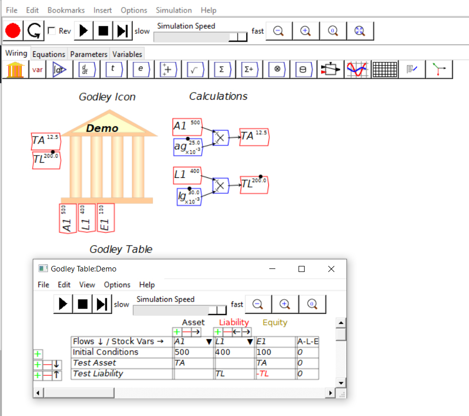
At the top of the Minsky canvas is the menu. The “File” selection allows you to open existing Minsky models and to save them. I haven’t used much more than that on the file menu.
If you use the hotkey equivalents, you will seldom need the “Edit” menu.
I have found setting up “bookmarks” can help when building a complex model. This takes you to the canvas position and magnification (zoom level) you were at when you created the bookmark.
“Options” allows you to change the background color; I use white because the screenshots used on the site look better. I go to “Options/Preferences to turn off the panopticon. The default is to display the panopticon in the upper right corner of the canvas. That shows where you are in relation to the entire canvas.
Help takes you to a table of contents of a tutorial which explains how Minsky works. The tutorial is old so some of the things in the tutorial are no longer in the newer versions of the program and other things may not work the same. Minsky is open source so you can examine the program source yourself or modify it.
Simulation Selections
Run the model using the next row of buttons.. The most useful of these selections are the three buttons to the left of the simulation speed slider. The left button starts the model running and will pause it if pressed while the model is running. The center button stops it and resets values to initial conditions. The right button steps the simulation through a single time period’s calculation.
If calculated values don’t appear in your variables, pressing the center, stop, button will perform the calculations for the starting values. It is useful to examine your model’s values at the start to make sure they make sense.
The speed slider will slow down the simulation. Sometimes, the model runs faster than you’d like so slowing the speed will allow you time to look around and watch the changes.
Zoom your view of the canvas in or out by using the buttons to the right of the speed slider. I generally use the center scroll wheel on the mouse instead. To display the entire model click the rightmost button; this is useful if you haven’t set up any bookmarks and lose your place in the model. Sometimes the sliders on the right side and bottom of the canvas (not shown in Figure 1) position you as though you clicked above or below the slider button. Clicking on the rightmost positioning button is faster than trying to find your position using the sliders.
Wiring Menu
Minsky opens on the “Wiring” tab below the simulation selections. You will use the wiring tab for most of your work on the canvas. You will not need most of the icon selections when creating the models shown on my website. Instead, type the names to create Variables and parameters. Press “*”, “/”, “+”, and “-” to create operations like multiply, divide, plus, and minus. .
A-L-E
To create the Godley icon and table shown in Figure 1, left click the Godley icon on the row of selections. When you move the mouse onto the canvas, the Godley icon will follow the mouse until you left click. Right click on the canvas icon to create the title, Demo.
The purpose of the Godley tables is to create sectors of an economy. Each sector has its own Godley table. On this website, these represent a macroeconomic sector, not an individual business or individual. Micro parts of an economy act differently than when considering the macroeconomy. Mainstream economists extrapolate microeconomies to the macro. This creates inaccuracies.
Double clicking the Godley icon on the canvas will show the Godley table on a separate inset screen. The “Asset,” “Liability,” and “Equity” columns define “stock” variables. Figure 1 shows the creation of the names of those variables A1, L1, and E1 at the “Stock Vars” line. If you need more Asset or Liability columns, click on the “+” just above the stock names. As you create the stock variables, their names will appear below the Godley Icon.
When the A-L-E column has an entry that is not zero, it indicates a violation of SFC. A-L-E means Assets minus Liabilities minus Equities. Just like a balance sheet in a business must satisfy those requirements, the model must meet those requirements as well.
Initial Conditions
The initial conditions row define the initial values of the stock variables. The flow variables below the initial conditions row will add to or subtract from the stock variable. You calculate the flow variables elsewhere on the canvas. The “Calculations” label identifies these in Figure 1.
The initial conditions must balance as well to ensure an accurate model.
Flow Variables
The original Godley table will have no transaction rows. In Figure 1, I created the two rows with the transaction descriptions, “Test Asset” and “Test Liability”. To create the rows, press the “+” key to the left of Initial Conditions. Create the flow variables by typing in TA, TL, and -TL as shown in Figure 1.
As you type in the flow variables, their names will appear to the left of the Godley icon.
Calculations
For the calculations, copy the variables used. Right click on the variable name at the bottom or the side of the Godley icon and select copy.
You can left click and drag to reposition anything on the canvas. By holding the left button and dragging, you can define a box. You can move anything within that box as a group by left clicking on an item in the box and holding it as you drag the mouse along the canvas.
To create the multiply icon, press the asterisk (*) key. Position the mouse at a blank location on the canvas and type in the names, lg and ag, to create the parameters; then press enter. (lg stands for liability growth and ag stands for asset growth.)
After typing in the variable name and pressing enter, an inset box appears. In the inset box where it says flow, click on the arrow to the right and select parameter. Set the initial value and press enter. For the demo, it doesn’t matter what those values are but I chose .025 and .03 so I could demonstrate two exponential curves that eventually intersect.
Create the wire connections by clicking and dragging on the circles that appear when the mouse hovers over the variable or parameter icon. You can only drag the wires one way.
Parameter Settings
You can change parameter values while running the model. To do this, position the mouse cursor over the parameter to change and press the left or right arrow on the keyboard.
Edit the parameter to set the size of the steps for each keypress. Right click on the parameter icon and select edit. Set the “Slider Bounds” max or min. The size of the steps is the last setting.
Don’t try to set these when creating the parameter. There is a bug in the software that creates its own limits and step size. After creating the parameter, select edit to set them the way you’d like.
Notes
Click on the icon that looks like a piece of paper and pencil to create the labels identifying the calculations, Godley icon, and the Godley table. (Positioning the mouse over the icon identifies the icon as “Note”.) As you move the cursor on the canvas, position the “Enter your note here” message where you’d like your label. Click to position it and double click to edit it.
Graphing
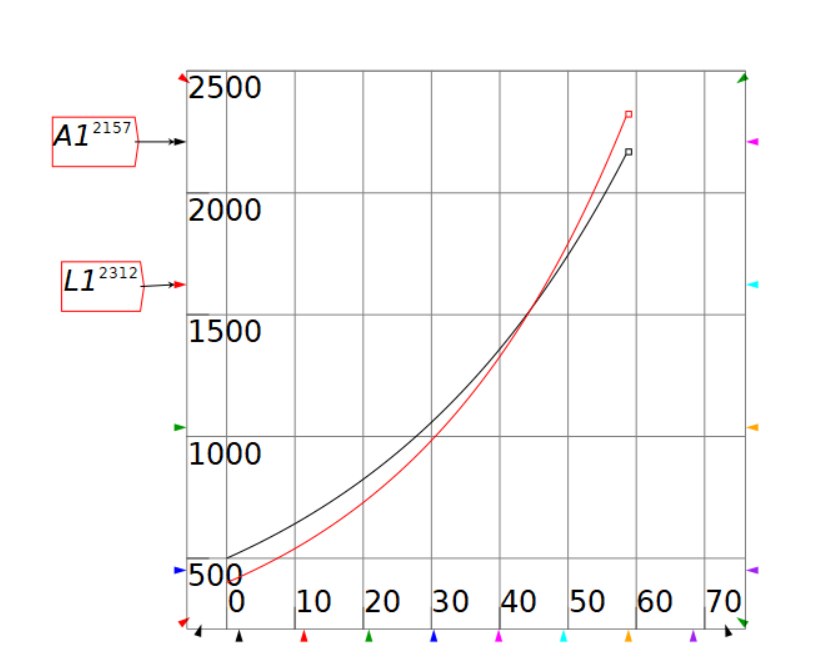
You can graph any of the variables easily. To create a graph, left click on the “Plot Widget” icon and move the mouse over a blank area of the canvas. Click again to place it. Adjust the size of the graph by dragging a corner. Catching the corner is sometimes difficult.
Next, copy the variables you want to graph. The variables graphed should have similar magnitudes or one of the variables will overwhelm the other. Figure 2 shows a graph of A1 and L1. L1 starts at 400 and A1 starts at 500. L1 overtakes A1 after about 45 years when both of them are about 1500.
You can give the graph a title and add labels to the axes by right clicking on the graph and selecting options.
Cycles
Figure 3 shows some interesting effects from interacting variables.
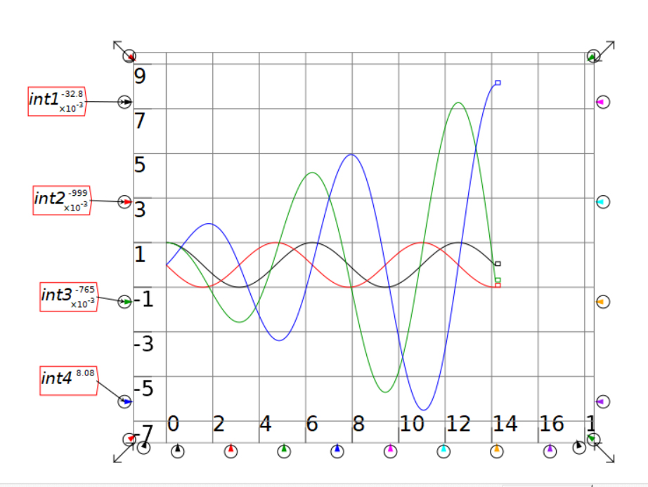
In Figure 3, note the red and black graphs. They are 90 degrees out of phase and the amplitude is constant. Now, note the blue and green graphs. They are 90 degrees out of phase and the amplitude is constantly increasing. The color of the arrow at the edge of the graph indicates what color the graph will be.
Cycle Calculation
Figure 4 shows the variables and parameters used to create the graph.
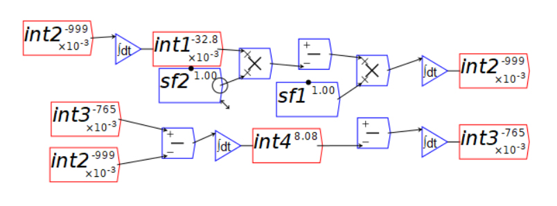
The Minsky program will not allow loops. If you route the output of one variable into the input of another variable and then route the output of the second variable into the first, the program will either crash or come up with an error message about infinite regress.
Godley tables is one way to create stock variables. Those are the columns on the table. In Minsky, you can create floating stock variables using the “Integrate” icon. Look at any of the variables in Figure 4 labeled intx. Create those by clicking on the Integrate icon and place the icon on the blank part of the canvas,
The integrate icon accepts input but does not pass it on until the program is run. It then passes the input only once until the program starts the next time period. In this way you avoid the infinite regress.
The upper part of the input triangle for the integrate icon accepts the calculation input while the lower part of the input triangle is the initial value. In this case, I set the initial value by right clicking the icon and selecting edit, then setting the initial value.
Notice the subtract operation that has nothing connected to the positive input. This converts the input to its negative at the output of the subtraction operation. You can change the parameters, sf1 and sf2, to notice the effect on the graph output.
Miscellaneous
Identify the rate of change of a variable by using the differentiate icon. I haven’t used it much so can’t give much insight on how best to utilize it.
The variable, t, is available if you have a function dependent on time. Minsky also has mathematical functions; sin, cos, ln, etc.; if you need them. It also has most of the common constants.
Equations Tab
Figure 5 shows the equation tab for the cycles calculations.
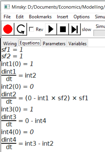
There is little need to look at the equations page. The same information is available and more clearly discerned by looking at the layout on the wiring page. I especially don’t look at the equations page on a large model.
In previous versions of Minsky the program would crash on large models when you looked at the equations tab and then tried to return to the wiring tab. I was also unable to see all the equations on large models.
Variables and Parameters Tabs
The variables and parameters tabs are useful mostly for quickly seeing the initial values all in one place. Otherwise, they are quite boring.
Final Thoughts
Minsky is a great program form economic modeling. This website will update the Models page as I find the time to write them up. It is faster to model an economy than to write about it.